I got a revise and resubmit on a recent paper. We noted that we had some missing data on some of the variables in our dataset. One of the reviewers suggested we address the missing data issue, which I have typically just managed using listwise/casewise deletion (a.k.a. complete-case analysis, which entails not including cases that have missing data on one of the variables in my models). I did, on a few papers in the past, use a variety of techniques to address missing data (back when I was using SPSS), but hadn’t done anything about this since switching to R. I saw this as an opportunity to learn a new technique – multiple imputation of missing data. It took a lot longer than I thought it might, but I got it to work. And since I did, I figured I’d share what I ended up doing in order to get it to work.
I was using R version 4.3.3 in RStudio 2024.04.7+748. The package I used is called “mice” version 3.17.0.
To illustrate how I did this (and I invite comments on suggestions if I did this wrong), I’m going to use my standard illustration dataset – the 2010 wave of the GSS. I’ll do this with two variables: one nominal and one ratio. The nominal variable I’m going to use is “BIBLE.” It asks participants to select the option that best reflects their view of the bible: (1) the literal word of a god, (2) the inspired word of a god, (3) a book of fables, (4) other. Here is the breakdown of the responses in 2010:
| Option | % |
|---|---|
| literal word of a god | 32.9 |
| inspired word of a god | 42.9 |
| a book of fables | 20.3 |
| other | 1.9 |
| missing/NA | 1.9 |
Typically, I would only report the percentages for those who answered the question and would ignore the missing cases, which make up 1.9% of the total participants in the GSS in that year – a total of 38 cases. But we’re going to impute those values.
The ratio variable I’m going to use is “WORDSUM,” which is the sum of how many of 10 vocabulary words that GSS participants were asked to define that they got correct. Here are the results for the “WORDSUM” variable:
| Option | % |
|---|---|
| 0 | 0.2 |
| 1 | 1.0 |
| 2 | 2.6 |
| 3 | 3.9 |
| 4 | 6.8 |
| 5 | 10.4 |
| 6 | 16.5 |
| 7 | 10.3 |
| 8 | 7.4 |
| 9 | 5.5 |
| 10 | 3.3 |
| missing/NA | 32.1 |
WORDSUM has quite a few cases missing – 32.1% of all the participants in 2010.
Let’s say I want to impute values for these individuals. Here’s how you can do that using the “mice” package in R.
First, of course, install “mice” and load the library. (Also, because I’ll be using it, go ahead and install “DataExplorer” as well):
install.packages("mice")
library(mice)
install.packages("DataExplorer")
library(DataExplorer)
The “mice” package has the ability to look for missing data in a dataset or dataframe, but it is only useful with smaller datasets. If you run this function on the entire 2010 GSS, it will check the whole dataset for missing cases and will take a long time. You’re better off subsetting the variable(s) you want and running this command on that subset. There is also another package that provides a nice visual illustration of missing cases: “DataExplorer”. I’ll show both. But, again, subset your dataset first before running either of these. Here’s what I did just for illustration purposes for this tutorial:
imputed <- subset(GSS2010, select = c(BIBLE,WORDSUM))
md.pattern(imputed)
To be clear, the first line above creates a new dataframe called “imputed” that is a subset of the GSS2010 and includes just two variables: “BIBLE” and “WORDSUM.” The second line calls the “missing-data pattern” function from “mice” for the newly created dataset. Note that I included just two variables in this subset for now. We’ll change this later. But the missing cases function in “mice” requires at least two variables in a dataframe to examine it because it is comparing and contrasting which cases are missing in the two variables.
Here’s the output:
     BIBLE WORDSUM
1365     1       1   0
641      1       0   1
22       0       1   1
16       0       0   2
        38     657 695
The output shows the two variables at the top and the number of missing cases at the bottom – 38 missing cases for the variable “BIBLE” and 657 missing cases for WORDSUM. The other values on the side are useful. Here’s what they mean: 1365 is the number of cases that have data for both variables; 641 is the number of cases that are missing only on WORDSUM but not BIBLE; 22 cases are missing only for WORDSUM but not for BIBLE, and 16 cases are missing in both variables.
It’s useful to run this function to make sure that “mice” can see that values are missing. There are situations when a variable has several values and they are not noted as missing (e.g., 9, 99, -1, etc.). It is also helpful to run this when you have additional variables to make sure there are existing cases for every missing case you have.
DataExplorer’s visual output is also useful:
DataExplorer::plot_missing(imputed)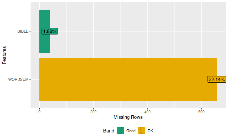
Both of these outputs should show that you have missing cases.
Now that you’ve confirmed that you have missing cases in those variables, the next step is to select the variables you want to impute missing values for as well as several other variables that can be used as the basis for generating the missing values. The authors of the “mice” package suggest you should have roughly 25 predictor variables for each target variable. Given how the imputation of missing values works, having variables that are related to the target variables but aren’t missing data is a good idea. It’s also a good idea to include basic demographic variables. Again, we don’t want a massive dataset as it will bog down the imputation process. Also, if there are IDs for the cases in your dataset, include that in the subsetted dataset because you’re going to want to bring the data back into your main dataset once you’re done imputing the missing values.
I’m going with three related variables for BIBLE: GOD, ATTEND, and POSTLIFE (i.e., view of a deity, frequency of religious attendance, and belief in an afterlife, respectively). And I’m going with three variables for WORDSUM: EDUC, AGE, WRKSTAT (i.e., years of education, participant’s age, and workforce status, respectively). I’m also including some other basic demographic variables: SEX, RACE, MARITAL, REGION, SIZE, CHILDS, SIBS, PAEDUC, MAEDUC, HOMPOP, INCOME, PARTYID, RELIG, FUND, PRAY, HAPPY, AND HEALTH. All of those plus ID. Here’s the code:
imputed <- subset(GSS2010, select = c(ID, BIBLE, GOD, ATTEND, POSTLIFE, WORDSUM, EDUC, AGE, WRKSTAT, SEX, RACE, MARITAL, REGION, SIZE, CHILDS, SIBS, PAEDUC, MAEDUC, HOMPOP, INCOME, PARTYID, RELIG, FUND, PRAY, HAPPY, HEALTH))You should probably run the same two checks on missing data on the full dataset. This is a good idea in case one of the variables you were thinking of using has lots of missing cases, which means it won’t be helpful for imputing values.
We have a few more steps before we actually impute the missing values. The next step is to make sure that the variables in the new dataset are the correct class (e.g., factor or numeric). This will matter when “mice” is looking to determine which method it is going to use to impute the data and when it is doing the imputation. This is particularly important with data imported from SPSS as it often gets a weird class like “haven_labelled,” which is meaningless to “mice” when it tries to figure things out. You can check and change the classes of your variables with the following code:
class(imputed$BIBLE)
imputed$BIBLE <- as.factor(imputed$BIBLE)
class(imputed$BIBLE)
class(imputed$WORDSUM)
imputed$WORDSUM <- as.numeric(imputed$WORDSUM)
class(imputed$WORDSUM)
# and so on for all of your variables in the new dataset
This next part is where I got really bogged down when trying to figure this package out. It took a lot of trial and error to come up with this solution, but it ultimately worked even though the package isn’t supposed to require this. Basically, you need to tell “mice” which variables you want it to impute missing values for and which ones you don’t. Though, in order to actually get all of the missing values imputed, you still have to let “mice” impute missing values for all of the variables in the dataset that are missing values. (I know this is a bit weird, but the first time I did this, I had some collinearity issues that caused some problems and ended up restricting “mice” to only imputing missing values for the target variables and no others, and this technique allows you to do that if you want to.) To do this, I created three items/lists and then used them to create a new dataframe:
vars_imp <- c("BIBLE","WORDSUM")   # the variables to impute
vars_aux <- c("GOD", "ATTEND", "POSTLIFE", "EDUC", "AGE", "WRKSTAT", "SEX", "RACE", "MARITAL", "REGION", "SIZE", "CHILDS", "SIBS", "PAEDUC", "MAEDUC", "HOMPOP", "INCOME", "PARTYID", "RELIG", "FUND", "PRAY", "HAPPY", "HEALTH")            # the variables for imputing
vars_id <- "ID" # ID
We then use the three items to create a new dataframe titled “df_imp”:
df_imp <- imputed[ c(vars_imp, vars_aux, vars_id) ]The next step is to have “mice” figure out which imputation method it is going to use for generating the missing values. There are four options: pmm, logreg, polyreg, and polr. These
- pmm – predictive mean matching (used with numeric data – i.e., interval/ratio)
- logreg – logistic regression imputation (binary data; factor variables with 2 levels)
- polyreg – polytomous regression imputation for undordered categorical data (factor variables with more than 2 levels
- polr – proportional odds model (ordered variables with more than 2 levels)
The “mice” package has a function that will go through the dataset and try to figure out which method to use with which variable. To not impute data for a variable, you can specify not to use a method with the second line of code. Here’s the code:
meth <- make.method(df_imp)
# meth["GOD"] <- ""
print(meth)
The first line of code will go through each variable, check to see if it is missing cases, and then try to decide which method it should use to impute the missing data. This is why setting the class for each variable in advance is important. The second line of code – commented out above – will tell “mice” not to impute any values for that variable. The third line of code lets you check the suggested imputation method. Here was my output:
BIBLEX WORDSUMX      GOD   ATTEND POSTLIFE     EDUC      AGE
   "pmm"    "pmm"    "pmm"    "pmm"    "pmm"    "pmm"  "pmm"
WRKSTAT      SEX     RACE  MARITAL   REGION     SIZE CHILDS
 "pmm"       ""       ""    "pmm"       ""       ""  "pmm"
SIBS   PAEDUC   MAEDUC   HOMPOP   INCOME  PARTYID   RELIG
"pmm"    "pmm"    "pmm"       ""    "pmm"    "pmm"    "pmm"
FUND     PRAY    HAPPY   HEALTH       ID
"pmm"    "pmm"    "pmm"    "pmm"       ""
Despite setting all of the factor variables as factor variables, “mice” still decided to use “pmm,” which isn’t accurate. I’m not sure why it didn’t get it right, but that’s okay. You can specify the method with this code:
meth["BIBLEX"] <- "polyreg"
meth["GOD"] <- "polyreg"
meth["POSTLIFE"] <- "polyreg"
meth["WRKSTAT"] <- "polyreg"
meth["MARITAL"] <- "polyreg"
meth["PARTYID"] <- "polyreg"
meth["RELIG"] <- "polyreg"
meth["FUND"] <- "polyreg"
If you do modify the method manually, check it again to make sure it worked. I checked mine and now it’s accurate.
We’re getting really close.
Now, we have to tell “mice” to calculate the predictors (a.k.a. variables) that it is going to use to do the imputations. Here’s the code to do that and then to check the results:
pred <- quickpred(df_imp, mincor = .05)
rowSums(pred[vars_imp, ])
The first line creates a new object called “pred” that is the number of predictor variables for each of the variables we want imputed values for based on a minimum correlation with the predicted variable of .05. The second line shows us how many variables it is going to use. Here is my output from the second line of code:
BIBLE WORDSUM
 20      21
Basically, “mice” is going to try to use most of the other variables in the dataset to impute missing values for BIBLE and WORDSUM. That should be fine.
Now, we get to run the actual imputation. This will create a new object that includes the results of the imputations. But it’s a long line of code with multiple pieces:
imp <- mice(df_imp,
            m      = 30,
            method = meth,
            predictorMatrix = pred,
            maxit = 30,
            seed   = 20250429)
The first line tells “mice” to create a new object, “imp”, which is a “mids” object. It is assigning to it the results from the function “mice”, which is going to process the “df_imp” dataframe. The “m = 30” line tells it how many multiple imputations. The method is the object we created above that specifies which imputation method to use. The predictorMatrix is also an object we created above that specifies the variables that are going to be used to predict our target variables. The “maxit = 30” part tells it how many iterations to run; 30 is probably overkill, but it is a recommended value. Finally, the “seed = XXXX” is basically any random number, but you should make note of it so others can replicate what you’ve done. I used the date when I was running the analysis the first time as my seed.
Assuming you’ve done everything correctly, once you get that code in place and run it, your computer is going to iterate for a while (it takes about a minute on my computer). Basically, it is running through lots of calculations and imputing values for the missing cases over and over. You should see something like this:
iter  imp   variable
1     1     BIBLE   WORDSUM GOD ATTEND POSTLIFE EDUC AGE WRKSTAT MARITAL CHILDS SIBS PAEDUC MAEDUC INCOME PARTYID RELIG FUND PRAY HAPPY HEALTH
1     2     BIBLE   WORDSUM GOD ATTEND POSTLIFE EDUC AGE WRKSTAT MARITAL CHILDS SIBS PAEDUC MAEDUC INCOME PARTYID RELIG FUND PRAY HAPPY HEALTH
.     .     BIBLE   WORDSUM GOD ATTEND POSTLIFE EDUC AGE WRKSTAT MARITAL CHILDS SIBS PAEDUC MAEDUC INCOME PARTYID RELIG FUND PRAY HAPPY HEALTH
30    30    BIBLE   WORDSUM GOD ATTEND POSTLIFE EDUC AGE WRKSTAT MARITAL CHILDS SIBS PAEDUC MAEDUC INCOME PARTYID RELIG FUND PRAY HAPPY HEALTH
Occasionally, when I run this, I get a warning message: “Warning message: Number of logged events: XXXX.” To see the logged events, you can use the following code:
print(imp$loggedEvents)The logged events can provide hints as to what went wrong if there are problems.
Now, if you’re like me, you went to all of this trouble so you could eventually get imputed values that you can then use in your analyses. How do we get those imputed values back into the original dataframe?
First, you have to convert the “imp” list into a dataframe. This code will do that:
df_analysis <- complete(imp, 1)This creates a dataframe/dataset called “df_analysis” that uses the first imputed value. You could pick any of the imputed values (1-30). This new dataframe has all of the original variables, but should now have the imputed values for the variables you specified. To check, just table the variables to see if there are any missing values now:
table(df_analysis$BIBLE, useNA = "ifany")
table(GSS2010$BIBLE, useNA = "ifany")
table(df_analysis$WORDSUM, useNA = "ifany")
table(GSS2010$WORDSUM, useNA = "ifany")
mean(df_analysis$WORDSUM, na.rm = TRUE)
mean(GSS2010$WORDSUM, na.rm = TRUE)
Checking the results, I now have no missing cases for BIBLE and WORDSUM and the mean for WORDSUM with the imputed values is almost identical to the mean for WORDSUM in the original dataset with no missing values. It worked!
Now, how do we get the data back into the original dataset so we can run whatever analyses we want?
First, I changed the names of the variables I wanted to pull back into the original dataset in the newly created dataset, adding “_imp” behind the name of the variable so I know that this is the variable with the imputed values:
df_analysis$BIBLE_imp <- df_analysis$BIBLE
df_analysis$WORDSUM_imp <- df_analysis$WORDSUM
Then, since I don’t want to pull back any of the other variables in the new dataset, I subsetted the new dataframe, keeping only three variables: BIBLE_imp, WORDSUM_imp, and ID (for matching with the old dataset).
df_analysis <- subset(df_analysis, select = c(BIBLE_imp, WORDSUM_imp, ID))
list(names(df_analysis))
With those three variables, I now just needed to join the variables to the original dataset, which is most easily done with the dplyr package:
library(dplyr)
GSS2010 <- GSS2010 %>%
  left_join(df_analysis, by = "ID")
Now, because I’m a little paranoid, I wanted to check to make sure that I have both the original missing data and can find the new imputed values in the new variables. So, a little checking:
which(is.na(GSS2010$BIBLE), arr.ind = TRUE)
GSS2010[2, "BIBLE_imp"]
The first line of code finds all of the cases that were missing for the variable BIBLE. The second line of code then lets me see the new imputed value for that case in the new variable, “BIBLE_imp” (just change the number for different cases). I just wanted to make sure everything worked okay. Sure enough, it did.
So, not the easiest thing in the world to do, but it’s manageable.
If you see that I did something wrong or have suggestions for improvement, please drop a comment.
![]()
Leave a Reply