One of the tasks I have to do regularly as part of my job is to compare two lists to see which items are missing on one list but not the other. I have been doing this by hand but figured there had to be a way to do this in Excel. I finally figured it out but don’t want to forget how to do it. So, I’m documenting it here so I can draw on this whenever I need to do it again.
Here’s the scenario. I have a list of “items” but every month or so I receive an updated list of “items” from someone else. During that month, some of the items on my list have been taken off and some have been added to it. Likewise, the same has happened to the other list that this other person sends me (I’m being really vague here because I work at a university and there are laws that govern academic records).
My list and the other list have to be kept synchronized but we have two separate databases that are used for this because… (argh, yeah). Anyway, what that means is that I have to compare the two lists and quickly find the items on one list but not the other and vice versa. Here’s how to do it quickly in LibreOffice Calc.
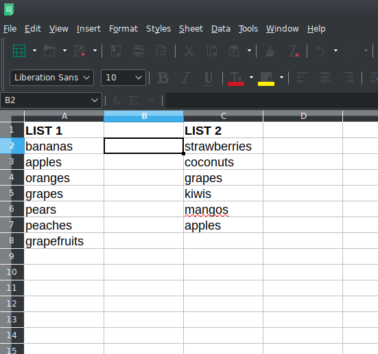
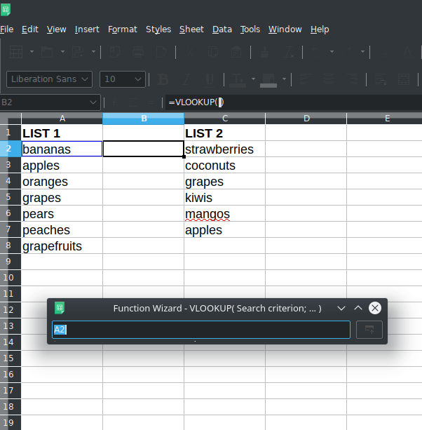
Here are two lists:
(NOTE: You can actually do this in two separate Calc sheets or within the same one.)
LIST 1 is in Column A and List 2 is in Column C.
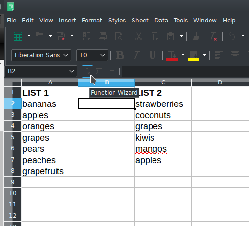
In Column B I am going to create a function that allows me to search all of Column C to see which of the items in LIST 1 show up in LIST 2. Click in Row 2 of Column B then click on the Function Wizard (or start typing):
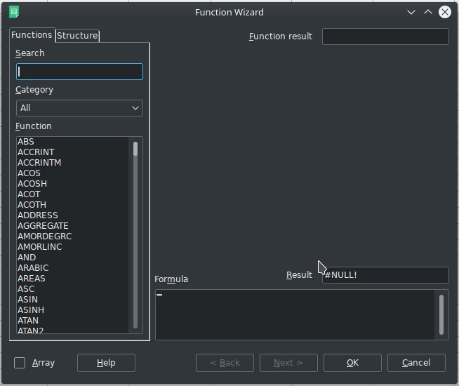
In the Function Wizard dialogue box, you’ll see this:
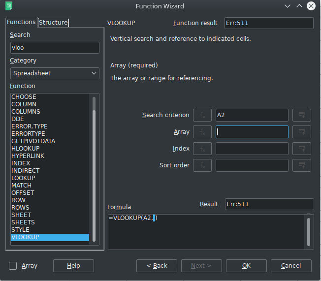
Search for VLOOKUP then double-click it and you’ll see this:
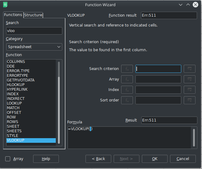
You now need to build the function. This is where I got confused, so I’m going to try to explain this carefully.
The first box is the “Search criterion.” Basically, this is what you want to find. In our example, let’s say that we want to see which items in List 1 are in List 2 (Hint: It’s apples and grapes.). So, we are going to put in the Search criterion that we want the software to search the items in column A or LIST 1. We do this by simply selecting cell A2 (you can do this by typing it in or by selecting it by clicking the button to the right of the box and then selecting A2 like I did below):
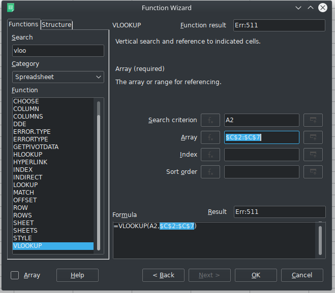
Next is the “Array” box. This is the content through which you want the software to search to find the items in LIST 1. Again, you can type this in or select it using the button to the right. However, there is an important change that you need to make here. If you select the array with your mouse and leave it as is, the values will change as you drag this formula down in Column B as it will assume you want to adjust the array as well. Since we don’t want to adjust the array but rather want to search through the same items in LIST 2, we need to put dollar signs before the letters and numbers in the Array which will lock the boundaries of the array into place so they don’t change when we copy the formula to other cells, as shown below:
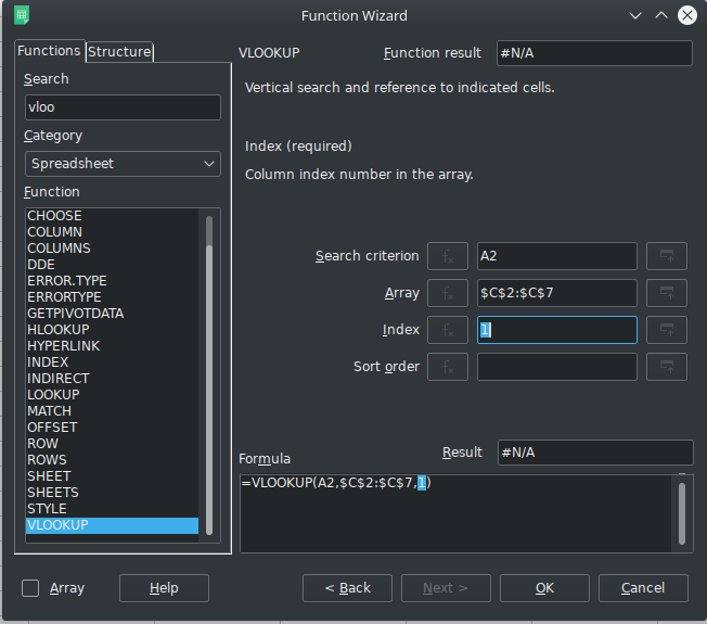
The next part is the part that threw me off for a long time in figuring this out. The “Index” is the column in the Array you want to compare to the Search Criterion. In this case, all you need to do is specify “1” since there is only one column. But, presumably, you could have an array made up of multiple columns and want to choose just the 4th column (so you would enter 4 in the Index). Someone in the comments clarified this. The “Index” is complicated. If you have just one column to which you are comparing your search criterion, the “Index” will return the value in that column that corresponds to your search criterion, which will always be the search criterion. In other words, if you were searching for “grapes” in Column 1 and only in column one, the “Index” will be “1” because there is only one possible value that can be returned, “grapes.” But imagine you have an “Array” that runs across four columns (e.g., A-D). The actual search criterion might be in column A, but you have something that corresponds to that value in column D, like “seedless.” You could have the “Index” return the value in the 4th column (i.e., .”D”) by putting “4” in the Index instead of “1”; “1” would return “grapes” if it finds it, “4” would return “seedless” if the software finds “grapes” in the array.
Okay, that was a rather long explanation. But, for my needs, I typically only need to enter “1” into the Index since I’m only looking through 1 column. Here’s how this looks:
Finally, the last box that is part of our function is the “Sort order” box. This tells the software whether the lists are ordered alphabetically or not. If they are not, enter zero (“0”). If they are, enter “1.” If you leave this blank, LibreOffice Calc thinks the lists are ordered. So, make sure you fill this out.
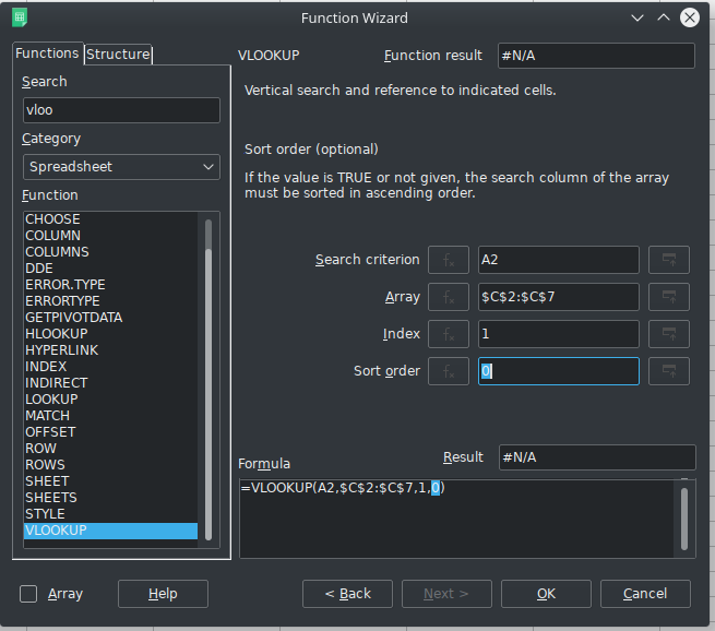
Once you’ve got that all entered, your formula should look like what I have above. Hit “OK” and it will search the Array C2:C7 for “bananas.” If it finds it, it will return “bananas.” If it doesn’t, it will return “#N/A” as shown below:
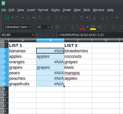
You can then, of course, drag this formula down. When it finds the item from LIST 1 in LIST 2 it returns that item. When it doesn’t, you get #N/A.
And there you have it. A LibreOffice Calc function for searching a list for a target and returning an indicator.
(NOTE: What I typically do after I have run this function is sort by the column where the function is located so I know which items are missing from LIST 1 and which are missing from LIST 2.)
![]()
