

In a different post on this blog, I showed how to use Vlookup to match lists. Someone commented on that post and indicated that it didn’t work with dates. It turns out, it does, but… There is a slight tweak required to make it work. So, if you want to learn how to use VLookup, first go to that previous post. Then come back here to see how this works with dates.
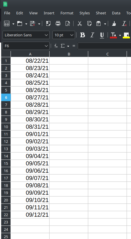
The issue with dates has to do with the format of the cells. To illustrate this, I created a spreadsheet and inserted a bunch of dates:

It’s important to make clear at this point that LibreOffice Calc, just like other spreadsheet software, has different “formats” for cells. Cells can be formatted as numbers, as text, as dates, etc. This is important because LibreOffice will treat cells with different formats differently. For instance, it’s pretty challenging to do numerical calculations with text (e.g., “apple” + 65 = ?). LibreOffice needs to know the “format” of a cell. That is the key to making vlookup work with dates.
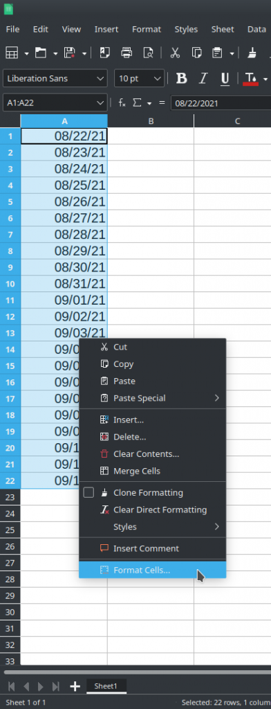
To check the format of a cell, all you need to do is right-click on it and select “Format Cells” (or Format -> Cells from the menus at the top of the screen):

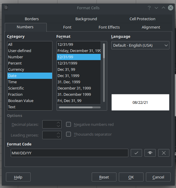
Obviously, if you’re working with dates, then the format for the cells should be “Date” and whatever specific date format you want:

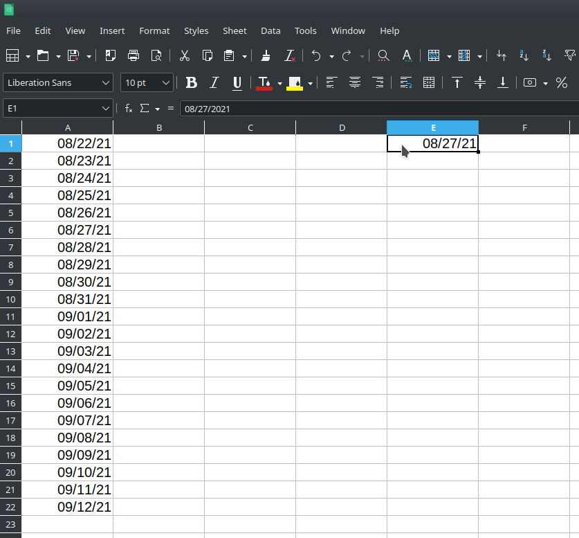
Okay, back to vlookup. To find a date in a list of dates, the value you are searching for also has to be a date in the Date format – ideally, they should be formatted identically. You can see in this spreadsheet, I inserted a date to search for in my list of dates:

The vlookup formula isn’t any different. In the cell just to the right of where I inserted the date I want to search for, I added my vlookup formula. Here’s what I put into my formula:
=VLOOKUP(E1,A1:A22,1,0)This formula calls the “vlookup” function. “E1” is the date for which we are going to search in the list of dates. “A1:A22” is the list of dates in which we are searching. The “1” after that says to use the first item in the list of items we are searching for (kind of a weird requirement). And the “0” tells LibreOffice Calc that the list is not alphabetized or sorted.
Once I put that formula in, LibreOffice Calc will search through the list to see if my date is in the list. I know that my date is there. And, typically, vlookup will return the matching date if it is there, so it should return “8/27/2021”. But, here’s what I get when I hit return on my formula:

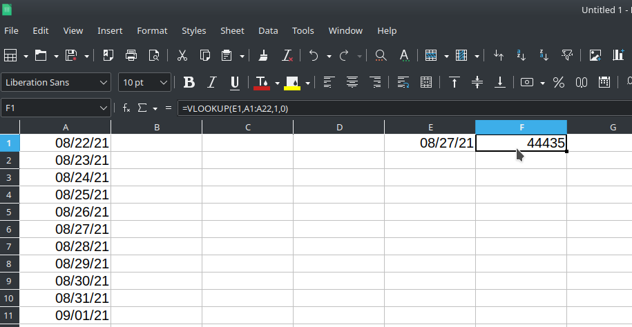
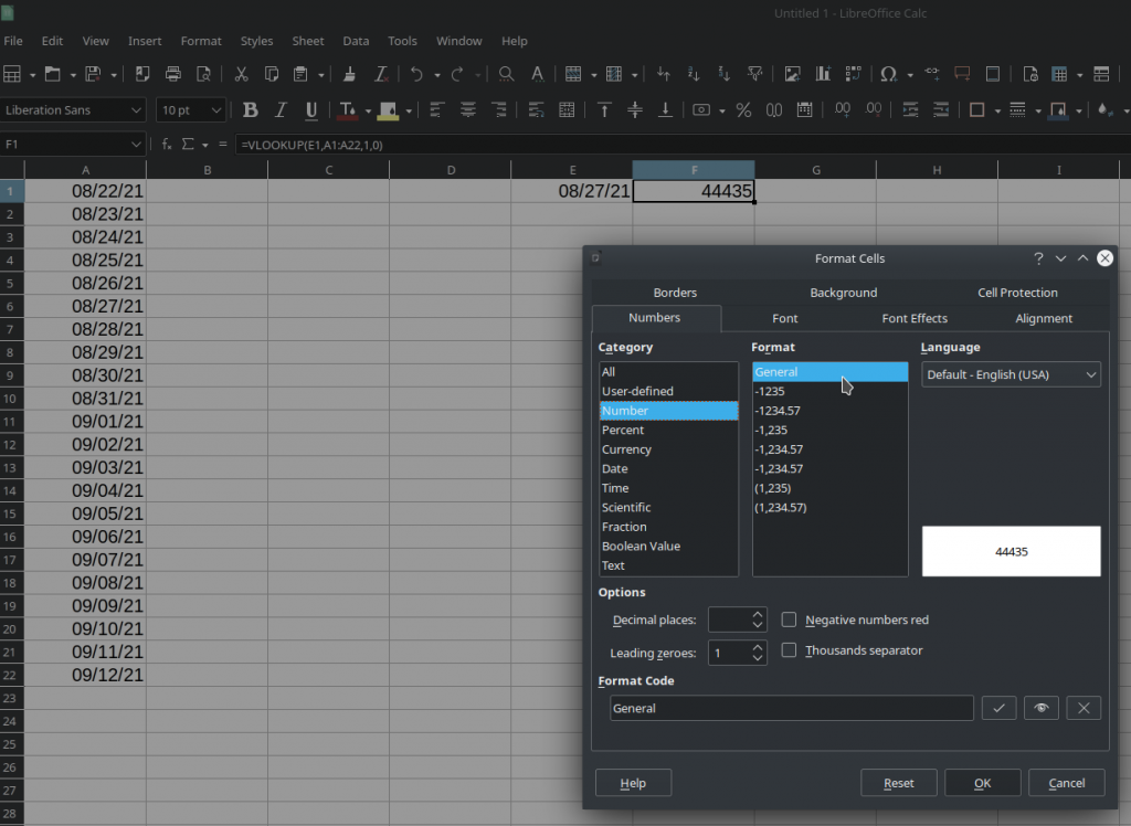
Rather than getting the target date, I get a weird number: 44435. Knowing a little bit about LibreOffice Calc, I quickly realized what the problem is: LibreOffice Calc doesn’t know that I’m searching for a date. It found the date, but the field where it is returning the value it found is currently formatted as a “Number,” not a “Date.” See:

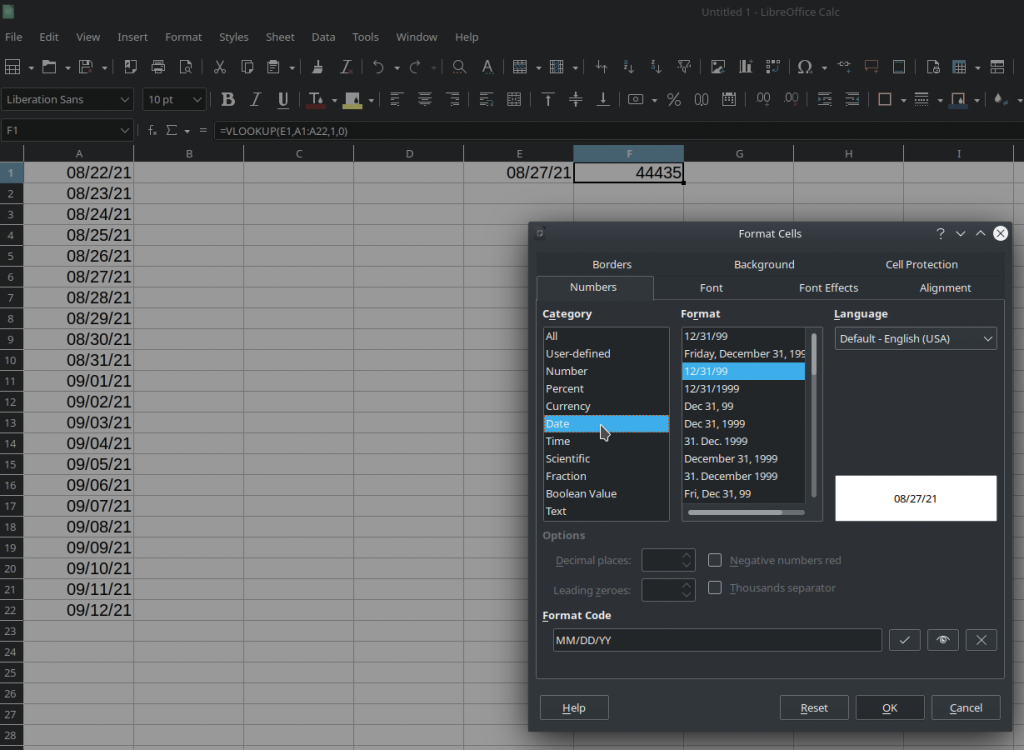
To show that it found the matching date, the vlookup cell also needs to be formatted as a Date. So, change the formatting for the vlookup cell:

And once you hit OK, you should now see the date it found:

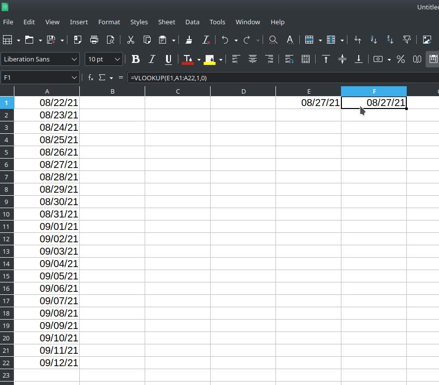
In short, yes, vlookup works with Dates. You just have to make sure that the cells where the vlookup formula is located are formatted as Dates not as Numbers and you’ll see which Dates match.
![]()
