

I haven’t used this feature of spreadsheet software as much as I probably should, but I have a spreadsheet I have been working with a lot lately and conditional formatting has been key to helping me orient myself in the spreadsheet. However, in the process, I realized that I am really a noob when it comes to conditional formatting. To help get myself up to speed, I created the following tutorial so I can reference it again in the future. (NOTE: I’m using LibreOffice 7.2.4.1 for this tutorial.)
Before I begin, what is conditional formatting? The basic idea is that you can change the look of a cell in a spreadsheet (or many cells) based on the contents of those cells (or other cells) without having to manually change the formatting of the cells. Instead, you “program” into the spreadsheet how you want cells to look assuming they meet specific criteria. Then, when you enter information into your spreadsheet, the cell formatting automatically updates to reflect the information in the cell.
Tutorial A – “Formula Is” Conditional Formatting
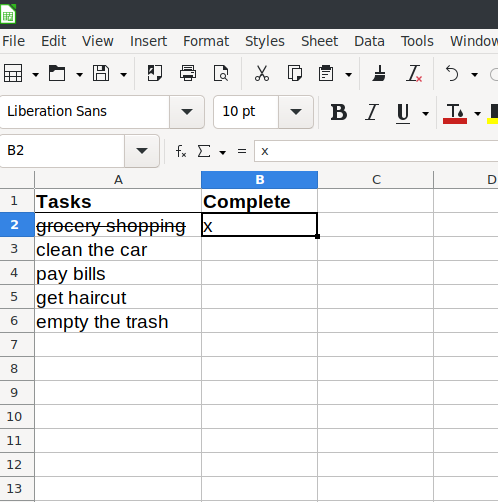
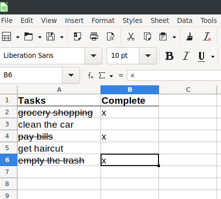
Let’s start with a very basic illustration. Let’s say I want to use a spreadsheet as a to-do list. Here’s how my spreadsheet looks, to begin with:

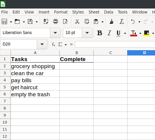
What I want to do is pretty simple. If I add an “x” to the Complete column for an item, I want that item to be crossed out. Effectively, I am going to change the font of the tasks to “strikethrough,” which crosses out the text. This way, I can quickly and easily discern which items are completed on my to-do list and which still need to be completed.
How do I set up the conditional formatting?
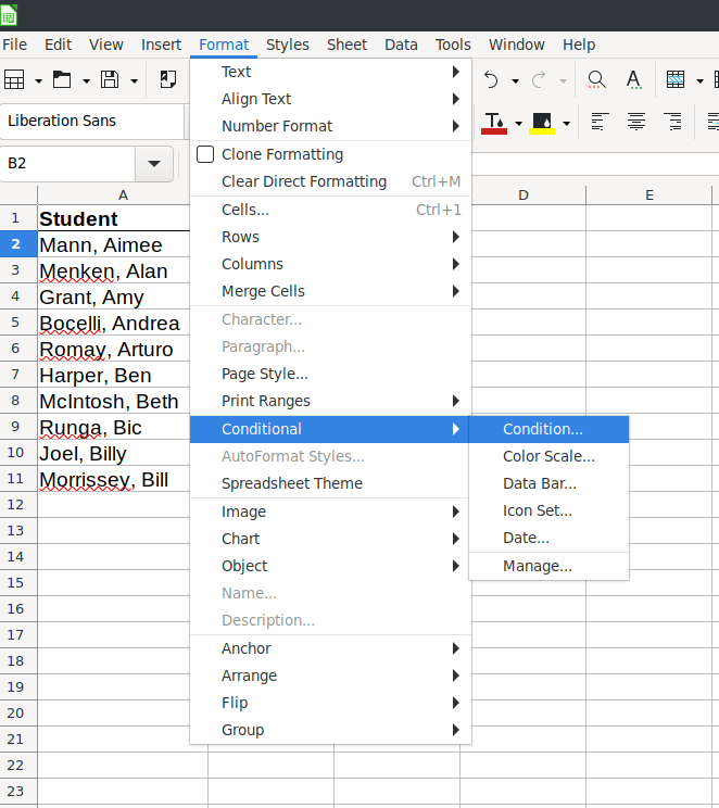
First, select the first cell (A2) that says “grocery shopping.” Then go up to “Format” on the menu and select “Conditional” -> “Condition.”


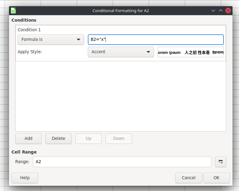
You’ll then get this window

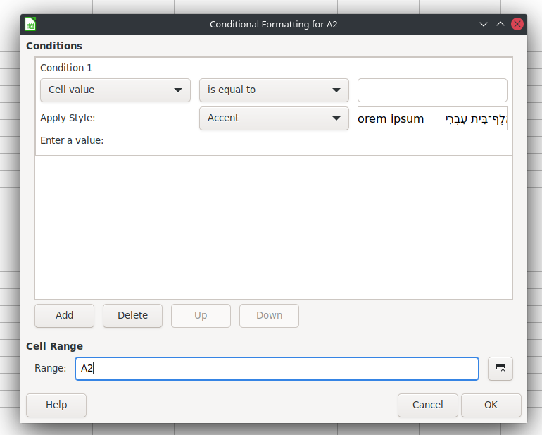
An explanation of the window is in order. At the bottom, the range of cells to which the conditional formatting will apply is included. Obviously, this can be set to a range of cells or just a single cell. Right now, I have it applying to just a single cell, A2.
Where it says “Condition 1” is where you will build your condition statement. If you click on the drop-down arrow where it says “Cell value,” you’ll see a couple of additional options:
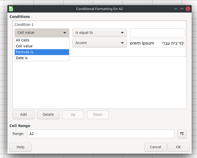
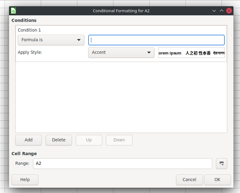
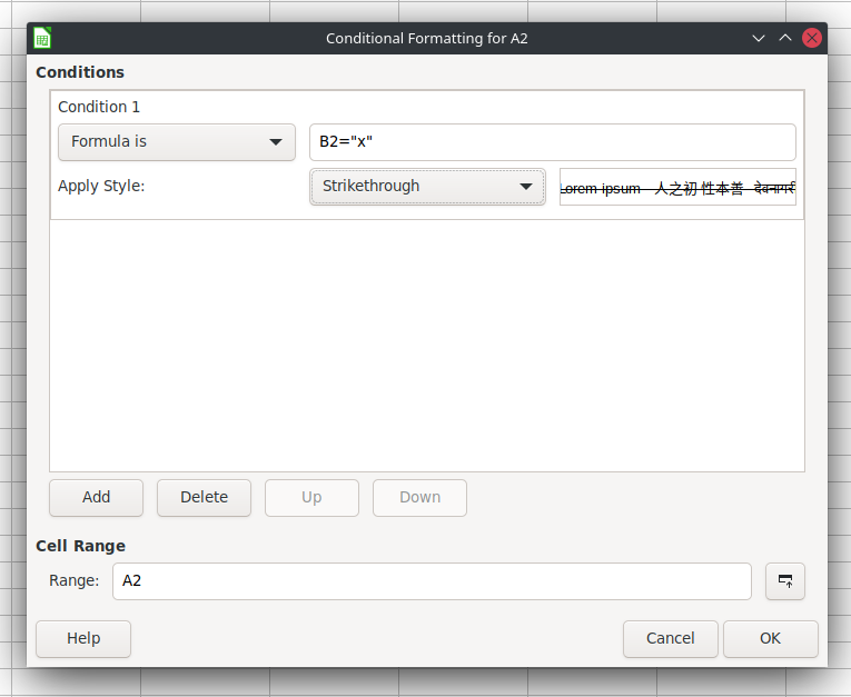
Those options are “Formula is” and “Date is.” This tutorial will cover two of the three options. For this one, we’re going to go with “Formula is.” The reason why we are going with “Formula is” is because we are going to use the information in a different cell, B2, to change the formatting in the current cell, A2. As the next tutorial will illustrate, you can also use the information in the same cell (e.g., A2) to change the formatting of that cell. So, select “Formula is.” You’ll notice that the window changes and you now just have a single box next to “Formula is” where you can enter your formula:
For our very simple to-do list, our formula will be pretty simple. We’re going to tell Calc to check to see if there is a lower-case “x” in B2. Here’s the formula: B2=”x”. (NOTE: If you want text or a character as part of your formula, it has to be inside quotes.) Here’s how it looks in the window:
Below that, we need to indicate how we want the formatting to change. If you click next to “Apply Style” where it says “Accent,” you’ll see a list of built-in formatting options:

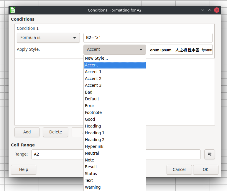
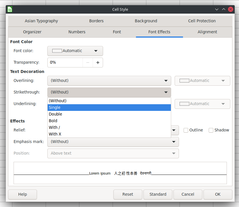
Since we want to have the text crossed out and that isn’t one of the built-in options, we’re going to select “New Style”. We’ll then get this window:

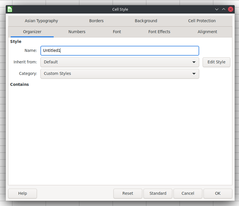
We actually only need to change two things. First, name the style. Since we are going with “Strikethrough,” let’s call this “Strikethrough.”
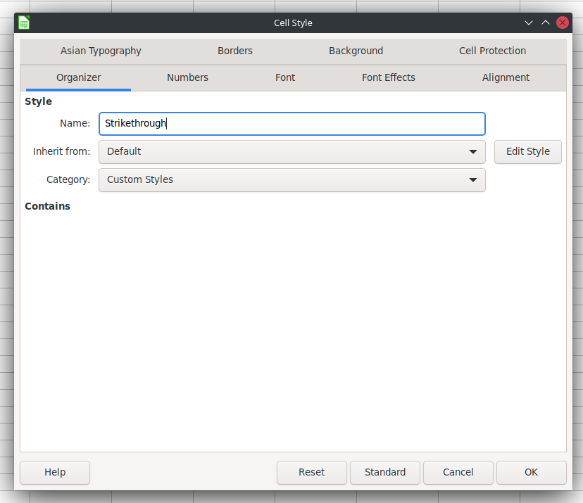
Next, Strikethrough is a Font Effect, so we click on the Font Effects tab and look halfway down the screen to where it says “Strikethrough.” By default, it says “(Without).” Click on that drop-down and select “Single” (or “Double” if that’s your fancy).
When you’re done, click “OK” and you’ll be taken back to the original Conditional Formatting window.

That’s actually all we need to do for now. Click OK on that window, and let’s test our Conditional Formatting. To test it, type a lower case “x” in B2 and hit “Enter” to see if your formatting works.

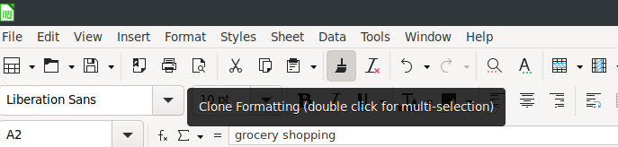
Okay, one more thing and the first part of this tutorial is done. We applied that conditional formatting to just one cell, A2. But we want it to apply to all the cells in that list. How do we copy the formatting and apply it to the others instead of having to repeat the process above? Select A2 and right-click. You’ll get a context menu. Look for “Clone Formatting” and select it.

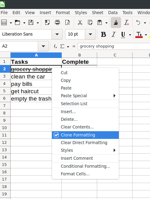
When you do, you’ll notice that the paintbrush icon on your toolbar is selected:

To apply the formatting you just cloned, select the cells you want to apply it to. Your cursor will change to a paint bucket. Click it over the selected cells and the conditional formatting will be applied to those cells. Now, test it. Add an “x” next to one of the other items to see if your conditional formatting is working:

Congratulations! You’ve successfully set up your first conditional formatting in LibreOffice Calc.
(NOTE: You can also apply the conditional formatting by indicating the cells to which the formatting should be applied in the Conditional Formatting window at the bottom. We indicated just A2 above, but you could include a range like A2:A6.)
Tutorial B – Conditional Formatting a Range with Colors
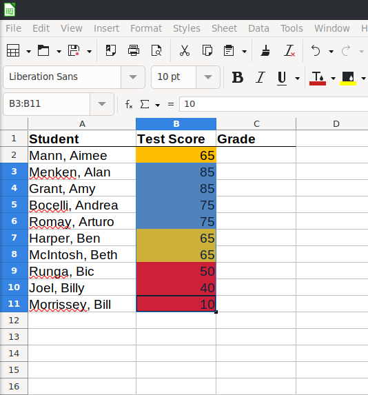
For this next tutorial, we’re going to get a little fancier. Nothing too crazy, but we are going to make the formatting conditional on the values in the cell and then apply background color to the cells. Our sample data are test scores.

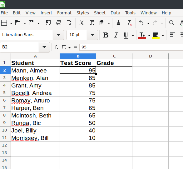
First, let’s select the top test score in B2 and go to the “Format” menu, then select “Conditional Formatting” -> “Condition.”

We’ll get the same window as we got in Tutorial A. But things are going to be different from here on. We’re going to set up a color code that reflects test score ranges so we can quickly see which students are doing well and which may need extra help. To do this, in that window, leave “Cell value” as is and select the next dropdown. We’re looking for “is greater than or equal to”:

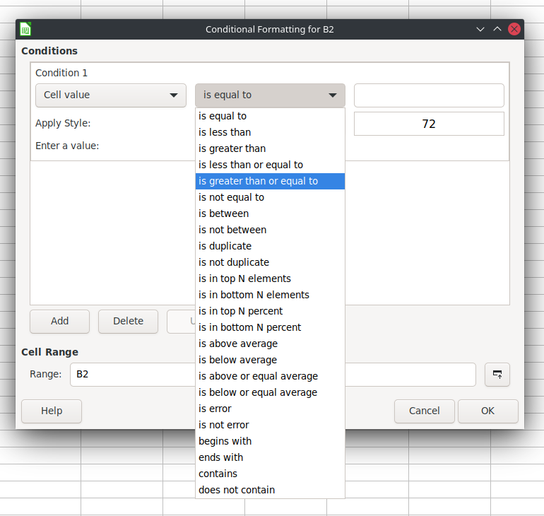
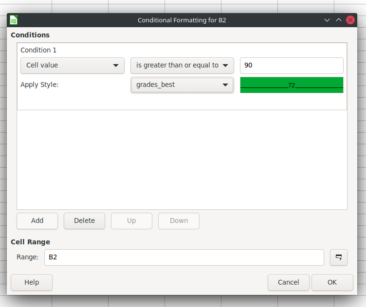
We want that option because the first condition we are going to enter is our top range of scores – 90 and up. Now, in the box next to that, enter 90. (NOTE: No need for quotes as this is a number, not text.)

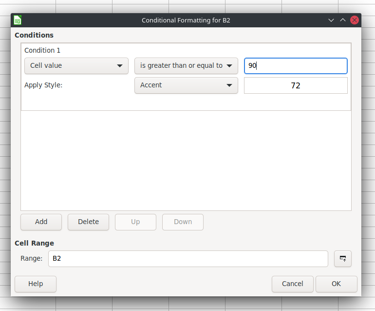
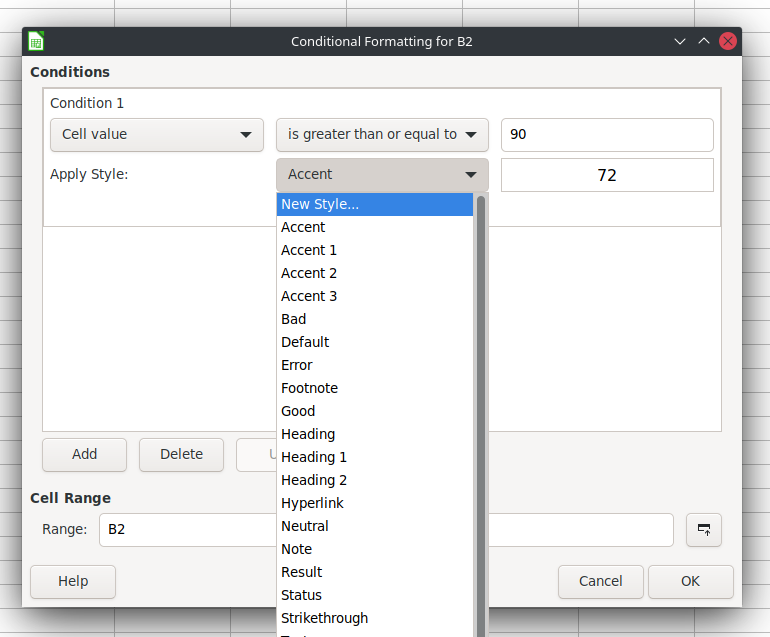
Now, the style. We are going to apply a colored background based on these ranges. So, in the dropdown next to “Apply Style” select “New Style”:
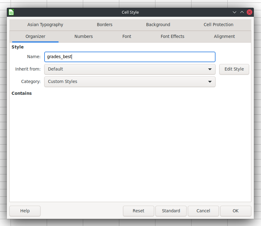
Like we did above, we’re going to name our style, something like “grades_best”.

Next, click on the “background” tab then select “Color” and you’ll see this:
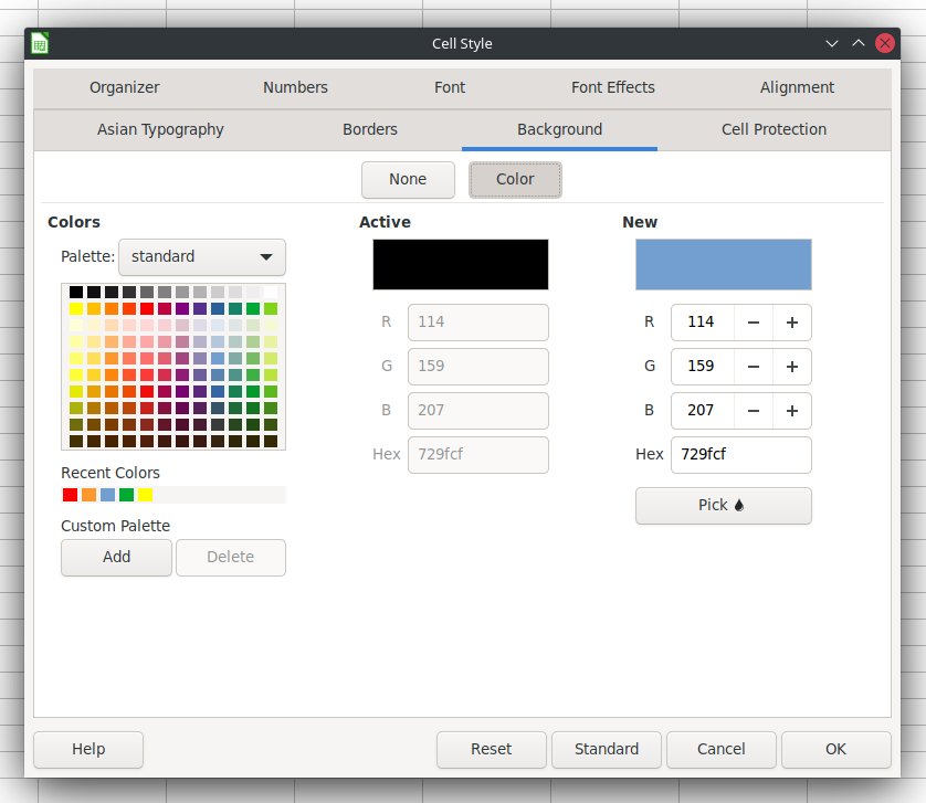
You can now pick the color you want to use as the background for that cell. I like green to mean that a student is doing well. So, I’m going with that:
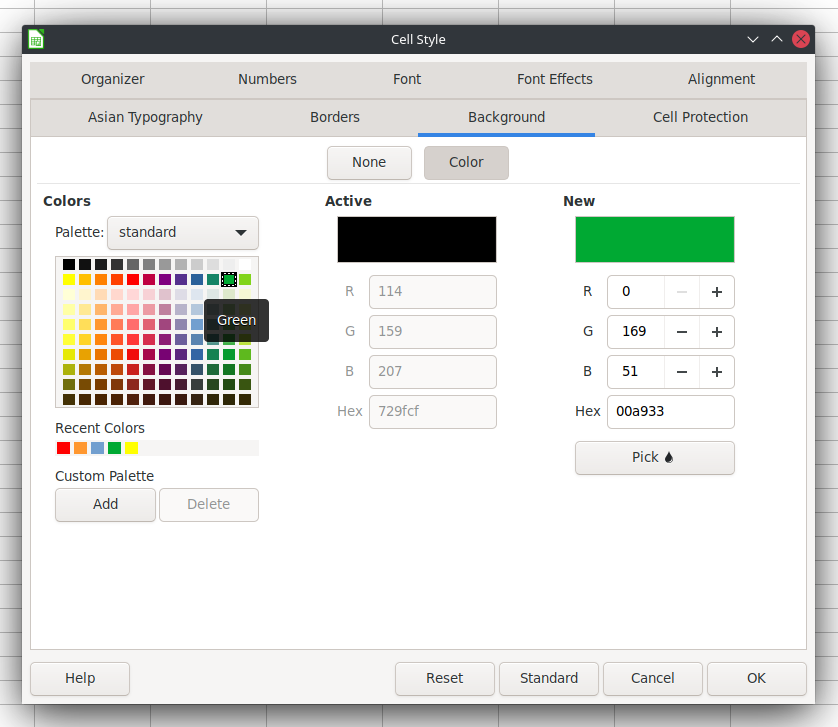
When you’ve picked your color, select “OK.” That will return you to the conditions window. We have our first condition, but we wanted to assign colors based on ranges. That means we need additional conditions. In that window, click on “Add.”

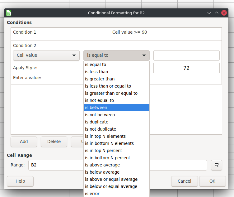
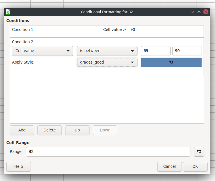
When you click on it, you’ll get “Condition 2.” We’re going to follow what we just did for Condition 1, but we’re going to change a couple of things. First, in the dropdown next to “Cell value,” we don’t want “is greater than or equal to” anymore as our next range will have upper and lower values. So, we want “is between.”
Now, think carefully about how this will work. Our first Condition was equal to or greater than 90. We want this one to range from 70 to 89. Thus, will need to set the two values as 69 and 90 so it includes all the values we want but excludes 69 and 90. Once you have that, follow the same steps above to set the background color you want. I went with blue for doing okay and named that style “grades_good”:
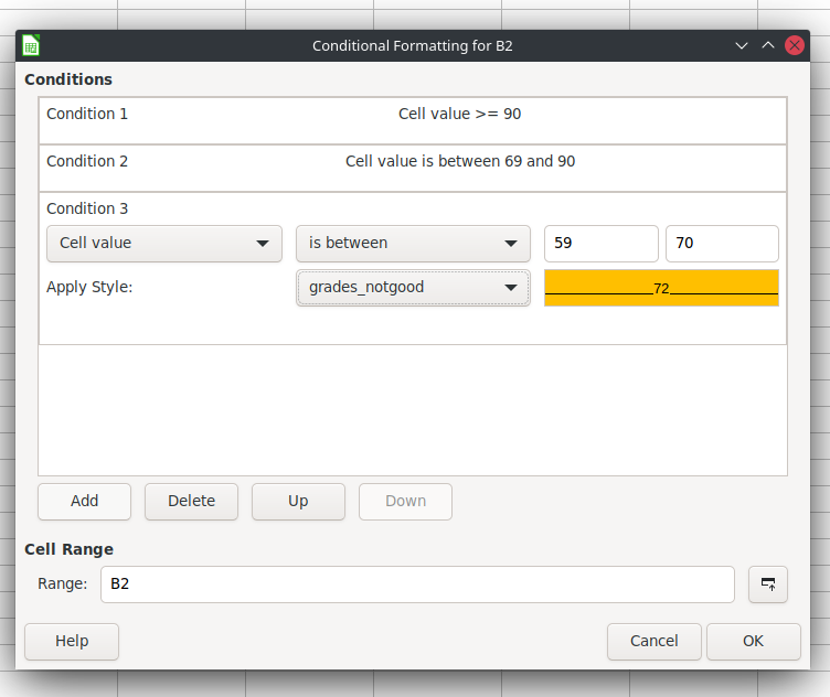
We’re going to set up two more conditions. One is going to be from 60 to 69 and is going to be orange. The last is from 0 to 59 and is red! Like this:
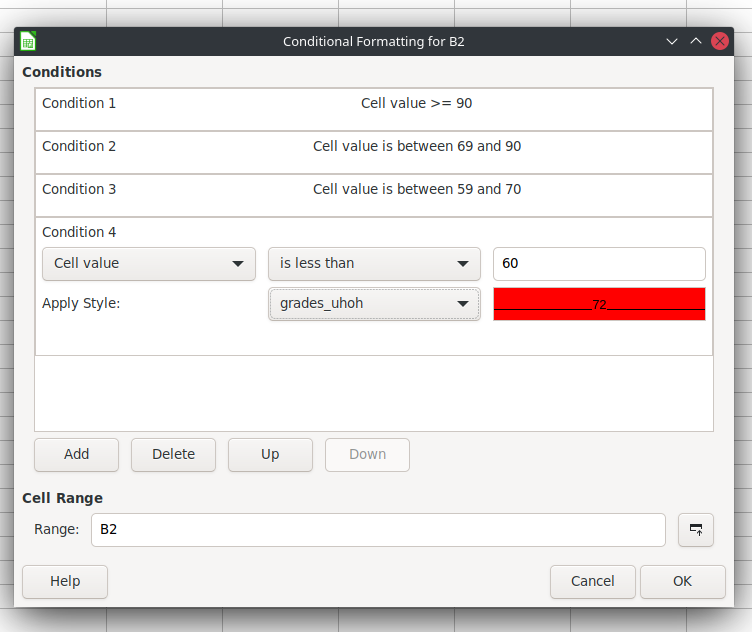
When you have all your conditions in, click “OK.” The background color for B2 should now change to match the conditions you created. You can test it by changing the values in B2 to make sure everything works.

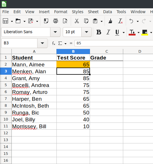
Now, as we did above, we can copy that conditional formatting and paste it to the other cells we want to have that formatting. Right-click B2 and select formatting then select the cells where you want to apply it and click with the paint bucket. All of those cells should now have the same conditions as B2.
There you go. That is how to use multiple conditions to format cells with a range of values.
Some Useful Notes
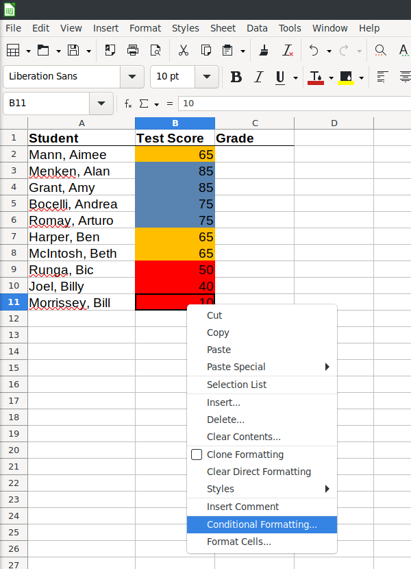
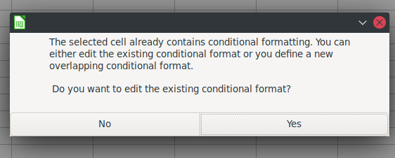
If you want to change the conditional formatting for a cell, be careful. If you right-click a cell with conditional formatting and select “Conditional Formatting” you’ll get this rather uninformative warning window:


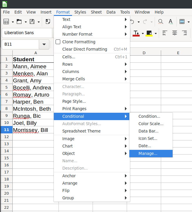
In this version of LibreOffice, whether you select “Yes” or “No” doesn’t seem to matter, it wipes out the current formatting. So, don’t do that. Instead, select the cell you want to modify, then click on the “Format” menu at the top of the window and select “Conditional Formatting,” but don’t select “Condition”! Instead, click “Manage” and that will pull up the existing conditions. You can then modify the existing conditions from that window.

![]()
