On my professional website, I use wordclouds from the text of my publications as the featured images for the posts where I share the publications. I have used a website to generate those wordclouds for quite a while, but I’m trying to learn how to use the R statistical environment and knew that R can generate wordclouds. So, I thought I’d give it a try.
Here are the steps to generating a wordcloud from the text of a PDF using R.
First, in R, install the following four packages: “tm”, “SnowballC”, “wordcloud”, and “readtext”. This is done by typing the following into the R terminal:
install.packages("tm")
install.packages("SnowballC")
install.packages("wordcloud")
install.packages("readtext")
(NOTE: You may need to install the following packages on your Linux system using synaptic or bash before you can install the above packages: r-cran-slam, r-cran-rcurl, r-cran-xml, r-cran-curl, r-cran-rcpp, r-cran-xml2, r-cran-littler, r-cran-rcpp, python-pdftools, python-sip, python-qt4, libpoppler-dev, libpoppler-cpp-dev, libapparmor-dev.)
Next, you need to load those packages into the R environment. This is done by typing the following in the R terminal:
library(tm)
library(SnowballC)
library(wordcloud)
library(readtext)
Before we begin creating the wordcloud, we have to get the text out of the PDF file. To do this, first find out where your “working directory” is. The working directory is where the R environment will be looking for and storing files as it runs. To determine your “working directory,” use the following function:
getwd()
There are no arguments for this function. It will simply return where the R environment is currently looking for and storing files.
You’ll need to put the PDF from which you want to extract data into your working directory or change your working directory to the location of your PDF (technically, you could just include the path, but putting it in your working directory is easier). To change the working directory, use the “setwd()” function. Like this:
setwd("/home/ryan/RWD")
Once you have your PDF in your working directory, you can use the readtext package to extract the text and put it into a variable. You can do that using the following command:
wordbase <- readtext("paper.pdf")
“wordbase” is a variable I’m creating to hold the text from the PDF. The variable is actually a data frame (data.frame) with two columns and one row. The first column is the document ID (e.g., “paper.pdf”); the second column is the extracted text. You can see what kind of variable it is using the command:
print(wordbase)
This gives you the following information:
readtext object consisting of 1 document and 0 docvars.
#  data.frame [1 × 2]
doc_id      text
<chr>        <chr>
1   career.pdf "\"      \"..."
R won’t show you all of the text in the text column as it is likely quite a bit of text. If you want to display all the text (WARNING: It may be a lot of text), you can do so by telling R to display the contents of that cell of the data frame, which is row 1, column 2:
wordbase[1, 2]
“readtext” is the package that extracts the text from the PDF. The readtext package is robust enough to be able to extract text from numerous documents (see here) and is even able to determine what kind of document it is from the file extension; in this case, it recognize that it’s a PDF.
The list can now be converted into a corpus, which is a vector (see here for the different data types in R). To do this, we use the following function:
corp <- Corpus(VectorSource(wordbase))
In essence, we’re creating a new variable, “corp,” by using the Corpus function that calls the VectorSource function and applies it to the list of words in the variable “wordbase.”
We’re close to having the words ready to create the wordcloud, but it’s a good idea to clean up the corpus with several commands from the “tm” package. First, we want to make sure the corpus is a plain text:
corp <- tm_map(corp, PlainTextDocument)
Next, since we don’t want any of the punctuation included in the wordcloud, we remove the punctuation with this function from “tm”:
corp <- tm_map(corp, removePunctuation)
For my wordclouds, I don’t want numbers included. So, use this function to remove the numbers from the corpus:
corp <- tm_map(corp, removeNumbers)
I also want all of my words in lowercase. There is a function for that as well:
corp <- tm_map(corp, tolower)
Finally, I’m not interested in words like “the” or “a”, so I removed all of those words using this function:
corp <- tm_map(corp, removeWords, stopwords(kind = "en"))
At this point, you’re ready to generate the wordcloud. What follows is a wordcloud command, but it will generate the wordcloud in a window and you’ll then have to do a screen capture to turn the wordcloud into an image. Even so, here is the basic command:
wordcloud(corp, max.words = 100, random.order = FALSE)
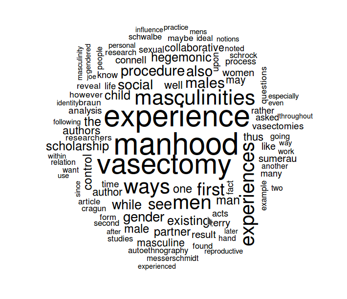
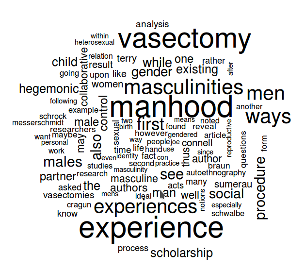
To explain the command, “wordcloud” is the package and function. “corp” is the corpus containing all the words. The other components of the command are parameters that can, of course, be adjusted. “max.words” can be increased or decreased to reflect the number of words you want to include in your wordcloud. “random.order” should be set to FALSE if you want the more frequently occurring words to be in the center with the less frequently occurring words surrounding them. If you set that parameter to TRUE, the words will be in random order, like this:
There are additional parameters that can be added to the wordcloud command, including a scale parameter (scale) that adjusts the relative sizes of the more and less frequently occurring words, a minimum frequency parameter (min.freq) that will limit the plotted words to only those that occur a certain number of times, a parameter for what proportion of words should be rotated 90 degrees (rot.per). Other parameters are detailed in the wordcloud documentation here.
One of the more important parameters that can be added is color (colors). By default, wordclouds are black letters on a white background. If you want the word color to vary with the frequency, you need to create a variable that details to the wordcloud function how many colors you want and from what color palette. A number of color palettes are pre-defined in R (see here). Here’s a sample command to create a color variable that can be used with the wordcloud package:
color <- brewer.pal(8,"Spectral")
The parameters in the parentheses indicate first, the number of colors desired (8 in the example above), and second, the palette title from the list noted above. Generating the wordcloud with the color palette applied involves adding one more variable to the command:
wordcloud(corp, max.words = 100, min.freq=15, random.order = FALSE, colors = color, scale=c(8, .3))

Finally, if you want to output the wordcloud as an image file, you can adjust the command to generate the wordcloud as, for instance, a PNG file. First, tell R to create the PNG file:
png("wordcloud.png", width=1280,height=800)
The text in quotes is the name of the PNG file to be created. The other two commands indicate the size of the PNG. Then create the wordcloud with the parameters you want:
wordcloud(corp, max.words = 100, random.order = FALSE, colors = color, scale=c(8, .3))
And, finally, pass the wordcloud just created on to the PNG file with this function:
dev.off()
If all goes according to plan, you will have created a PNG file with a wordcloud of your cleaned up corpus of text:

NOTE:
To remove specific words, use the following command (though make sure you have converted all your text to lower case before doing this):
corp <- tm_map(corp, removeWords, c("hello","is","it"))
Or use this series of functions, which is particularly helpful for removing any leftover punctation (e.g., “, /, ‘s, etc.):
toSpace <- content_transformer(function (x , pattern ) gsub(pattern, " ", x))
corp <- tm_map(corp, toSpace, "/")
corp <- tm_map(corp, toSpace, "@")
corp <- tm_map(corp, toSpace, "\\|")
Source Information:
Reading PDF files into R for text mining
Building Wordclouds in R
Word cloud in R
Removing specific words
Text Mining and Word Cloud Fundamentals in R
Basics of Text Mining in R
For Advanced Wordcloud Creation:
There is another package that allows for some more advanced wordcloud creations called “wordcloud2.” It allows for the creation of wordclouds that use images as masks. Currently, the package is having problems if you install from the cran servers, but if you install directly from the github source, it works. Here’s how to do that:
install.packages("devtools")
library(devtools)
devtools::install_github("lchiffon/wordcloud2")
letterCloud(demoFreq,"R")
You can then use the “wordcloud2” package to create all sorts of nifty wordclouds, like this:
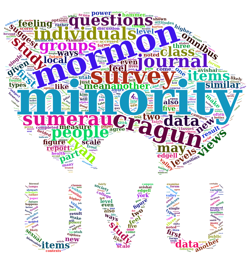
Before you can use wordcloud2 to create advanced wordclouds, you need to convert your data (after doing everything above) into a data matrix. Here’s how you do that:
dtm <- TermDocumentMatrix(corp)
m <- as.matrix(dtm)
v <- sort(rowSums(m),decreasing=TRUE)
d <- data.frame(word = names(v),freq=v)
The data matrix is now contained in the variable “d”. To see the words in your frequency list ordered from most frequently used to least frequently used, you can use the following command. The number after “d” is how many words you want to see (e.g., you can see the top 10, 20, 50, 100, etc.)
head(d,100)To create a wordcloud using wordcloud2, you use the following command:
wordcloud2(d, color = "random-light", backgroundColor = "grey")And if you want to create a wordcloud using an image mask (the image has to be a PNG file with a transparent background, you use the following command:
wordcloud2(d, figPath = "figure.png", backgroundColor = "black," color = "random-light")Note: Source for directions on wordcloud2 are here and here; though see here for converting your corpus into a data matrix, which is what you have to use to create these fancy wordclouds.
NOTE: Color options for wordcloud2 are any CSS colors. See here for a complete list.
![]()
